Maths
| Site: | Learn : Loughborough University Virtual Learning Environment |
| Module: | WSRESTF - Foundation Studies |
| Book: | Maths |
| Printed by: | Guest user |
| Date: | Tuesday, 7 July 2026, 8:53 AM |
Description
1. Why do I need maths?
2. Taylor series
3. Complex numbers
4. Differential equations and Laplace transform
5. State space analysis
6. Fourier transform and spectral density functions
7. Matrices and Eigen value analysis
8. Statistics and applied probability
1. Why do I need maths?
Why is an understanding of engineering maths necessary? The CREST MSc is not a heavily mathematical programme, but some elements do require mathematical treatment.
This unit has been developed to reflect the level of mathematics that underpins the more technical modules (Wind I, Solar I, Integration, Wind II and Solar II in particular). Note that you will not always be required to manipulate the equations etc yourselves. The intention is that you can understand what is being done and why. Also please note that this Unit is intended for revision of what many of you will have already been taught as part of your previous training and education.
Some self-assessment questions have been added to help you judge you current knowledge and understanding, but it will quickly become apparent on reading the material whether you are sufficiently familiar with these areas of mathematics. Don't feel under pressure to complete all of these. If you do encounter difficulties, don't panic! There is a wide range of more basis mathematics self-study material at a more introductory level, which can be viewed and downloaded from the Open Learning Project. You are recommended to visit the "Workbook" section first. Note: this is only available to registered students.
When you look at the extensive list of work-sheets don't be intimidated - you are only looking for the topics covered in our material with which you are having difficulties, and these are easily found. The only exception is State Space analysis, which is the modern engineering approach to control modelling, and relates to the material on linear systems (and hence linear differential equations and the associated topic of Laplace transforms).
Work through the sheets as you need, and don't be afraid to ask for help from the people at the Mathematics Support Centre. If in doubt about the relevance of a particular bit of mathematics, please directly approach the CREST staff concerned with the more technical modules.
Study tips
This unit consists of a series of compact study notes and self-test questions. You are recommended to study the unit in the following sequence:
1. Tackle the pre-test questions, where available, to gauge your prior knowledge. This will indicate whether you need to concentrate on a particular unit.
2. For each topic, work through the study notes sequentially. Make sure that you understand any worked examples.
3. Where available, you may wish to tackle the self-test questions as they occur in the sequence. If you encounter difficulties, return to the study notes and focus on the relevant topics before re-visiting the self-test.
4. If you are stuck, arrange to discuss specific difficulties at a study group meeting or with a member of staff. 5. If you are still unsure, contact a foundation tutor via the Learn server or directly by email.
2. Taylor series
Why?
You will not have to use Taylor Series yourselves, but it is a common way in which useful approximations are generated (eg that sinq can be approximated by q for small angles). There are occasions when lecturers will use this to provide a simpler formulation (eg expressions relating to extreme winds in the Wind II module).
What?
If a function f(x) is differentiable up to nth order in some neighbourhood of a point x = a, then in the neighbourhood, the function can be represented by a power series in (x - a).
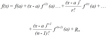
For many functions the remainder term Rn → 0 as n → ∞, and so we can write
 (1.1)
(1.1)
This series expansion is known as the Taylor series. For the case of a = 0 it is known as the Maclaurin's series.
Some important series easily derived are for the exponential, cosine and sine functions.

Series expansions are widely used in engineering to provide approximations to functions.Sufficient accuracy is often achieved by taking just the first two terms of the series. If (x - a) < < 1 then higher powers will contribute little.
Say we wish to express the value of a function for small displacements h from an operating point a. Then h = x - a and equation (1.1) becomes
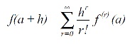
Taking just the first two terms (sometimes referred to as linearisation) gives
![]()
If we take as an example f(x) = xn, then
![]()
and it is clear that all powers of h greater than 1 have been discarded. Provided h < < 1 such approximations are reasonably accurate.
3. Complex numbers
Why?
Complex numbers are generally used in engineering, electrical engineering and quantum mechanics. They provide a system for finding the roots of polynomials used in theoretical models for the investigation of electrical current, wavelength, liquid flow in relation to obstacles, dynamos and electric motors, and the manipulation of the matrices used in modelling.
What?
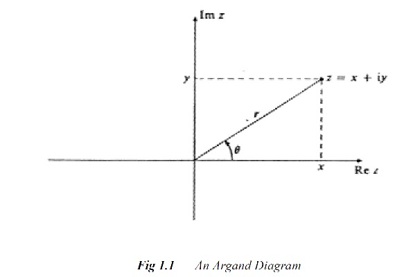
The complex number z = x + iy can also be written in modulus argument form
![]()
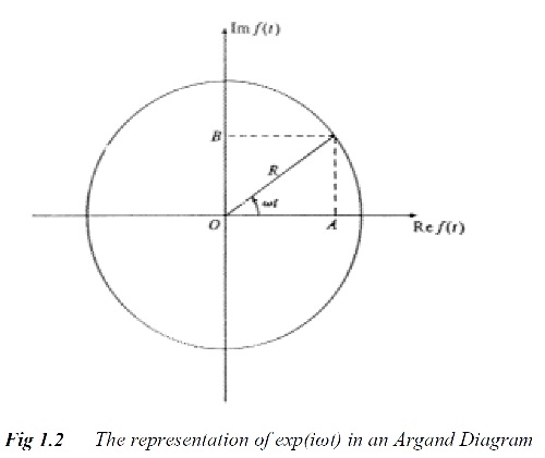
The real part, Re z = x = r cos θ and the imaginary part, 1mz = y = r sin θ. Complex numbers can be shown as points on an Argand diagram.
Standard rules exist defining, addition, subtraction, multiplication and divisions of complex numbers.
We can show that there exists the following convenient alternative form of equation (2.1):
![]()
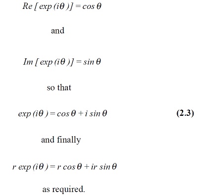
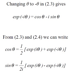
Just as a series expansion for exp (x) was calculated, (equation (1.2)), so we can write down the series for exp (iθ) as
Taking the real and imaginary parts we get:
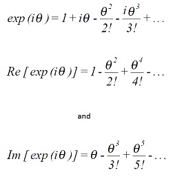
Comparison with equations (1.3) and (1.4) gives us that
From (2.2) complex numbers are straightforward to multiply:
![]()
By extension, for z with unit modulus,
![]()
This is de Moivre's theorem. It is often written in the alternative form:
![]()
Equation 2.2 also provides a very useful framework for the analysis of periodic systems.
For example, if θ = ωt, where ω is an angular velocity, then the function
![]()
has real and imaginary parts which undergo sinusoidal variations with amplitude R and
period 2π/ω (although out of phase by π/2).
4. Differential Equations and the Laplace Transform
Why?
Differential equations arise in thermal analysis (as in Solar I) and to describe water waves (as in the Water Power module). You will not be expected to solve differential equations as part of the course but it is important that you understand where the presented solutions come from, and the role of boundary conditions. Laplace Transforms are not explicitly used in the MSc but they do underpin basic control analysis.
What?
4.1 First-order equations
4.2 Second-order equations
4.3 The Laplace transform
Definitions
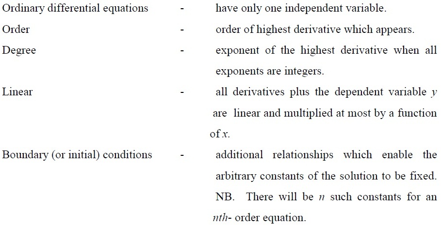
4.1. First-order equations
The general first-order equation can be written as
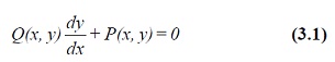
If the equation can be rewritten in the form
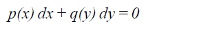
the variables are said to be separated and the solution is given trivially as
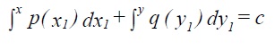
Generally this will not be the case. The solution sought can be written as
![]()
Differentiating this with respect to x gives
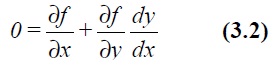
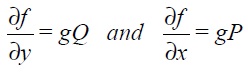
By comparison with the original equation (3.1) we get
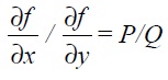
If the original equation (3.1) pre-multiplied by a function g(x, y) is to result in the form given by (3.2) then
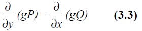
since
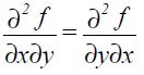
we get
For the particular case of g (x, y) constant the original differential equation is known as exact and the solution can be written down as
![]()
where the function h(y) is chosen so that
Alternatively the solution
![]()
where
may be easier to evaluate.
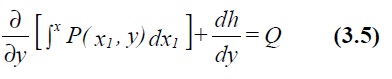
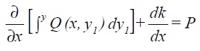
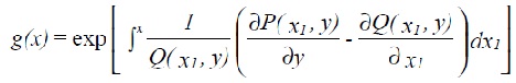
If the equation is not exact, an integrating factor g (x, y) must be found. Expanding equation (3.3) gives
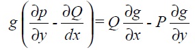
If P is substituted from the original equation we get an equation for g:
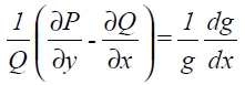
For common occurring cases where the LHS of (3.5) is a function of x only the solution can be obtained directly by integration as
4.2. Second-order equations
Second-order equations occur frequently in the description of dynamical systems with springs, damping and inertial forces. Very often these will also be linear. The general case of importance is
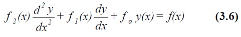
where, in dynamic analysis, f(x) on the RHS is the forcing function. A special case has f(x) = 0. A solution of (3.6) is known as the particular function, whilst a solution of (3.6) with f(x) = 0 is called the complementary function. The general solution of (3.6) is the sum of these two. Solutions of (3.6) are often of the form
![]()
where λ1 , λ2 and c are fixed numbers and A and B the two arbitrary constants to be fixed through application of the boundary conditions. For many dynamic systems (3.6) can be further simplified so that f0, f1 and f2 become constants, ie
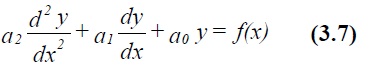
If f(x) is zero or takes a simple form we can proceed as follows. Assume the complementary function is of the form
![]()
This results in
![]()
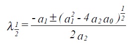
which is clearly satisfied if
![]()
This expression, known as the auxiliary equation, is solved to give λ (two solutions in general) λ1 and λ2
Since the differential equation (3.7) with f(x) = 0 is linear we can write down the complementary function (in this case the general solution for f(x) = 0) as
![]()
4.3. The Laplace transform
The Laplace transform is an integral transform given by
![]()
It is a linear transformation which takes x to a new, in general, complex variable s. It is used to convert differential equations into purely algebraic equations.
Some examples are given in the table below:
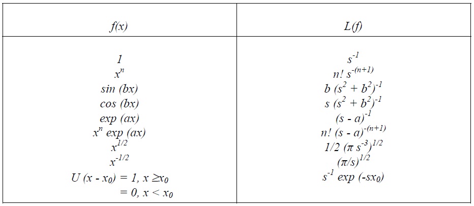
Deriving the inverse transform is problematic. It tends to be done through the use of tables
of transforms such as the one above.
For application to differential equations we start by evaluating L(df/dx) using integration by
parts, the result is
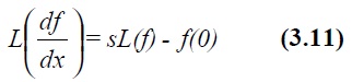
This process can be repeated for ![]() etc, giving
etc, giving
Hence the Laplace transform of any derivative can be expressed in terms of L(f) plus derivatives evaluated at x = 0. It is thus possible to rewrite any differential equation in terms of an algebraic equation for L(y).
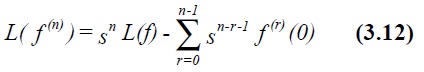
Four useful properties of Laplace transforms can be established.
4.3.1 Control theory applications
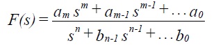
Laplace transforms are widely used in classical control theory. The independent variable is often taken as time t. In many applications the transformed differential equation will turn out to be the ratio of two polynomials in s, for example
If required this can be split by partial fractions to give
![]()
where the inverse transform L-1 can be found separately for each element. Hence
![]()
Often in control theory the inverse transform is not taken since much can be concluded (regarding stability etc) from the form of F(s).
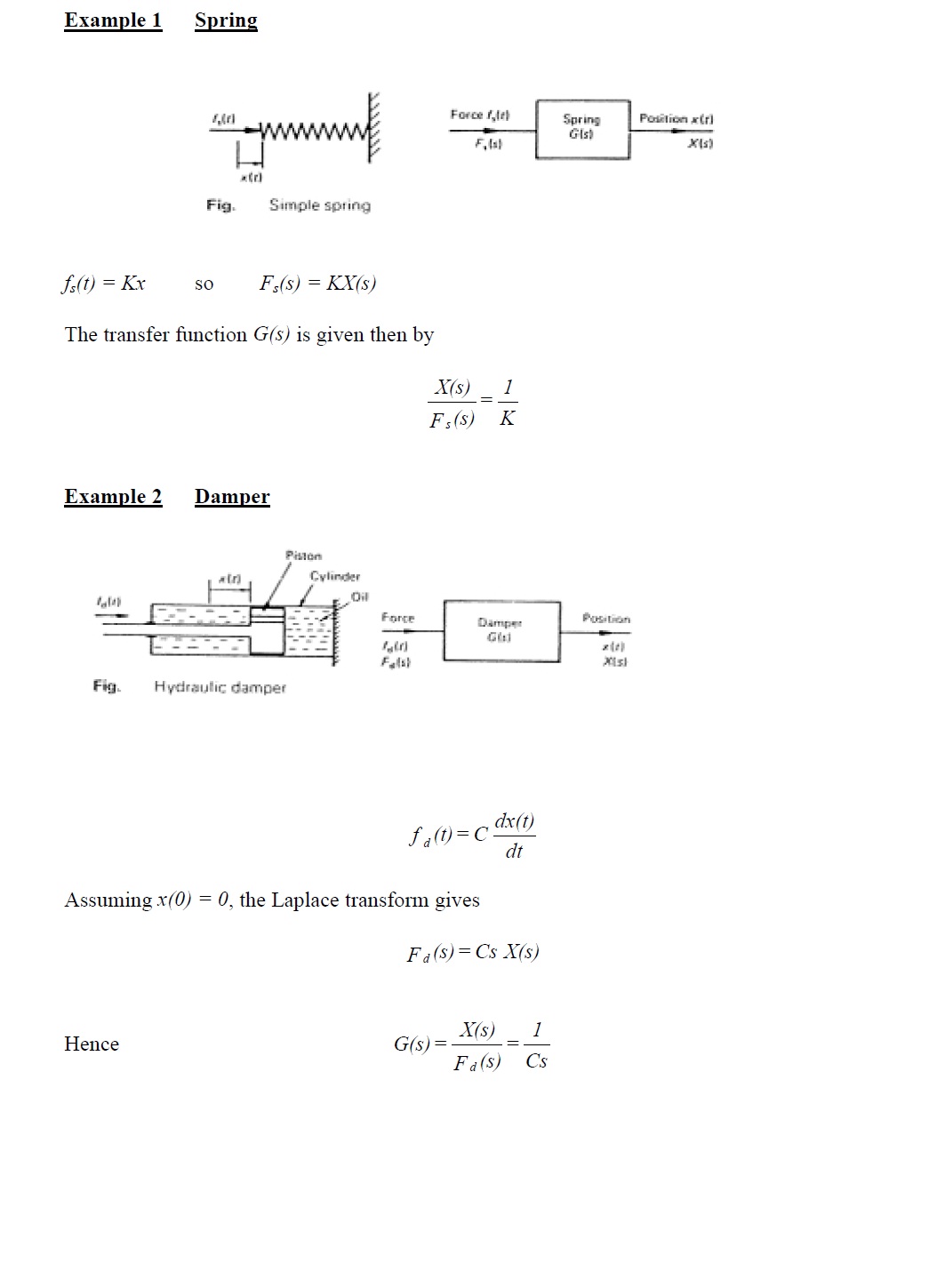
The transfer function of a linear system is defined as the ratio of the Laplace transform of the output of the system to the Laplace transform of the input to the system. It is denoted by G(s) or H(s). The linear assumption means that the properties of the system (eg G(s)) are not dependent on the state of the system (value of t or s).
For transfer functions, the initial conditions are assumed to be zero so that
![]()
Differential equations are transformed into the Laplace domain simply by replacing ![]() etc. The resulting transfer function can then be written
etc. The resulting transfer function can then be written
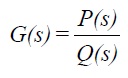
where P and Q are polynomials in s. The properties of G are determined by the roots of Q (s) = 0 (which is known as the characteristic equation).
NB. These roots are referred to as poles of the system since G(s) becomes infinite at these values of s. The order of the system is the order of Q(s).
4.3.2 Calculating transient response to a step input
The approach developed above can be used to calculate the transient response of linear systems. First order systems are straightforward to analyse but not particularly interesting. We will concentrate here on second order systems.
The output of a system is often denoted by c(t) and its Laplace transform by C(s) with the
input being u(t) and U(s) respectively.
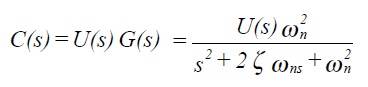
The Laplace transform of a step input is 1/s and so
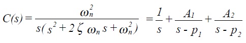
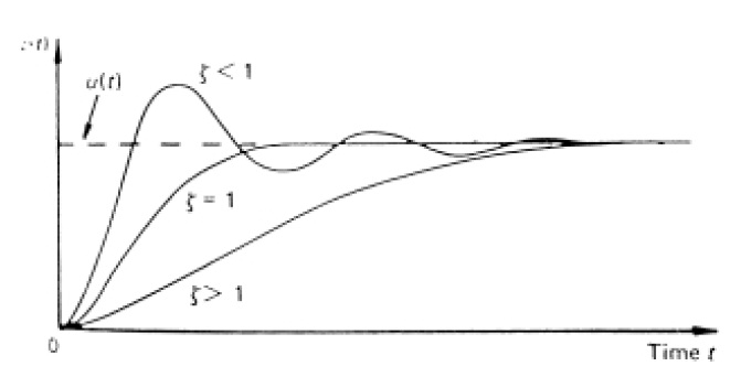
using partial fractions where A1 and A2 are constants and p1 and p2 are the roots of the characteristic equation. Hence, taking inverse transforms,

The nature of the response depends on the nature of the roots, which is determined by the damping factor ζ. The figure below shows the form of step response for a second order system.
5. State Space Analysis
Why?
This brief note is simply to introduce the concept of state space analysis so that you will recognise the terminology. You will not be expected to apply this approach yourselves.
What?
Fundamentally, state space analysis is a rewriting of the equations of motion (or more generally equations describing an arbitrary system) in terms of first order differential equations. The dependent variables of these equations are known as the state variables. For an nth order system (nth order DE) there will result n first order equations and so there will be n state variables needed to describe the system. The decomposition into first order DEs is not unique and neither therefore is the choice of state variables. Often the choice will be determined by pragmatism (ie a simpler set of equations results) or physical meaning (ie the state variables have a clear physical interpretation).
A vector, having as its components the state variables (which are functions of time), is known as the state vector. At any time it represents the state of the system.
Once the initial state is known together with the inputs, the state of the system for all future times can be calculated.
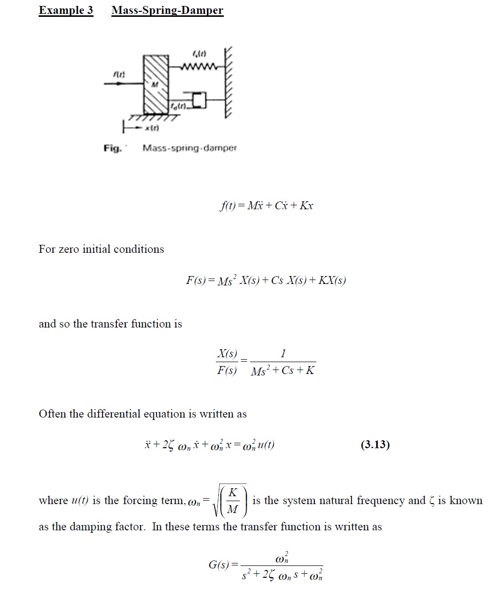
The mathematical space which encompasses all possible values of the state vector is known as the state space; hence the term: state space analysis. The dimension of the state space is the order of the system. Take for example the mass-spring-damper equation (3.13). This can be written as a pair of first order DEs:
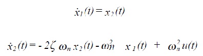
where x1(t) ≡ x(t) , the position at time t and x2 (t) ≡ x!(t), the velocity at time t. The variables x(t)and x!(t)are the state variables; they completly describe the system.
The pair of equations can be written in matrix notation as follows:
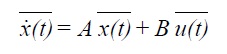
where x(t)is the state vector and
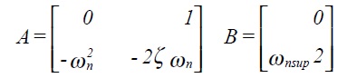
and u(t) is the forcing vector.
An advantage of state space analysis, in contrast to transfer function analysis, is that it can be extended from single input-single output systems to multi-variable systems with many inputs and outputs and also that it can deal with non-linear systems.
6. Fourier Transform and Spectral Density Functions
Why?
These notes are simply to assist you in understanding what a spectral density function is. You will not be expected to manipulate such functions, but they are a handy way to represent wind speed variation (as in Wind I and Wind II modules).
What?
Harmonic functions
Harmonic functions (written as eiωt or cos (ωt)) are attractive from an analytical point of view for a number of reasons: they are straightforward to differentiate, integrate and multiply; moduli are easily evaluated and each contains only one frequency. The last property will be found to be useful in the context of analysing systems which are characterised by a fundamental (resonance) frequency. Complexity can be dealt with through superposition.
Technically, the harmonic functions can be shown to the mutually orthogonal and complete (any reasonable function can be expressed as a linear combination of them). If the period of f(t) is T, then mutual orthogonality means
![]()
If we take f(t) = cos (2πnt/T) with integer n, it can be shown to be orthogonal by integrating
over the range (-T/2, T/2).
Since cos (2πnt/T) is an even function, linear combinations will always be even.
A more general set of functions is then required to give completeness. As a function can be
expressed as the sum of an even and an odd part, the suggested set of functions is:
![]()
for integers n and m.
It is straightforward to show that the orthogonal property still applies.
A particular linear combination of the above set (which also has the desired properties) is
![]()
This is attractive in that it can be written as simply exp (i 2πnt/T).
Fourier series
A Fourier series is an expansion of a function in terms of its Fourier components as suggested by the above discussion.
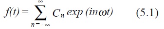
The constants Cn are known as the Fourier coefficients, ω = 2π/T is the fundamental
frequency.
If a function f(t) is known, the Fourier components can be projected out by pre-multiplying
by exp (-im ωt) and integrating from -T/2 to T/2.
Fourier series can be differentiated and integrated term by term.
6.1. Fourier transforms
The Fourier transform (or Fourier integral) is obtained formally be allowing the period T of the Fourier series to become infinite. Instead of only integer frequency contributions (as in the Fourier series) a continuous function of frequency results. From equation (5.1) we can write down
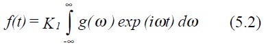
where K1 is an arbitrary constant. By analogy, the Fourier coefficients Cn become a continuous function g(ω), ie
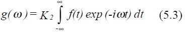
K2 is also arbitrary, although the product K1 K2 is fixed. It is conventional to take K1 and K2 as 1/ 2π .
Equation (5.3) is known as the Fourier transform and (5.2) the inverse Fourier transform.
The function g(ω) is called the spectrum of f(t).
It can be noted that as an integral transform it is similar to the Laplace transform but that both limits of integration are infinite.
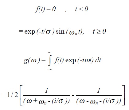
Example 1: Fourier transform of exponential decay function f(t) = 0 for t < 0 and f(t) = exp (-λt) for t≥ 0 with λ > 0.
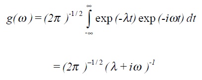
NB: Complex contour integration is required to derive this, however it is easily checked using the inverse transform.
Example 2: Fourier transform of Gaussian or normal distribution function, (zero mean and standard deviation σ).
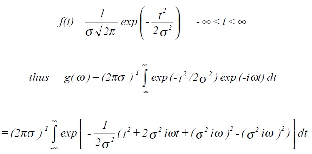
which can be rewritten as
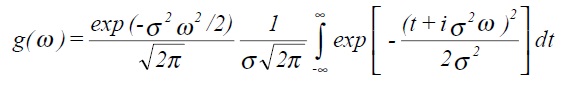
Finally this can be shown to give
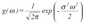
which is also a Gaussian distribution with zero mean but with standard deviation equal to 1/σ.
ie σω σt = 1
The narrower in time an impulse is, the greater the spread of frequency components.
6.2. Properties of the Fourier transform
These are listed without proof:
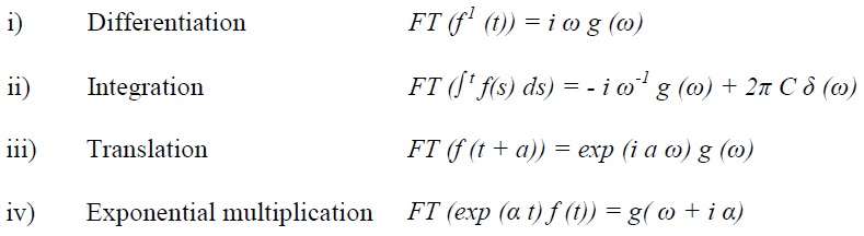
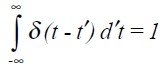
where α may be real, imaginary or complex and 2π Cδ (ω) is the Fourier transform of the constant of integration associated with the indefinite integral, and δ(ω) is the delta-function given by
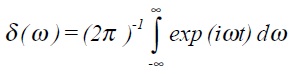
6.3. Properties of the Dirac delta-function
Combining the definitions of the Fourier transform and the inverse Fourier transform we can write (suitably arranged)
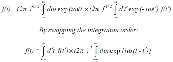
This is very instructive since the second term, which in the delta-function notation can be written simply as δ (t - t'), has the property of selecting out just one point from the infinite integral and assigning a finite value to the result. This leads to an alternative definition of the delta-function, namely
![]()
except for t = t' where the function is infinite or more rigorously
6.4. Parseval's theorem
Parseval's theorem can be stated as:
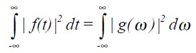
Its proof regimes use the properties of the δ-function.
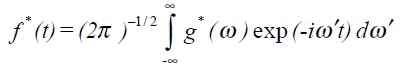
In brief, if we take the complex conjugate of (5.2), the inverse transform
The intensity I of a function is defined to be
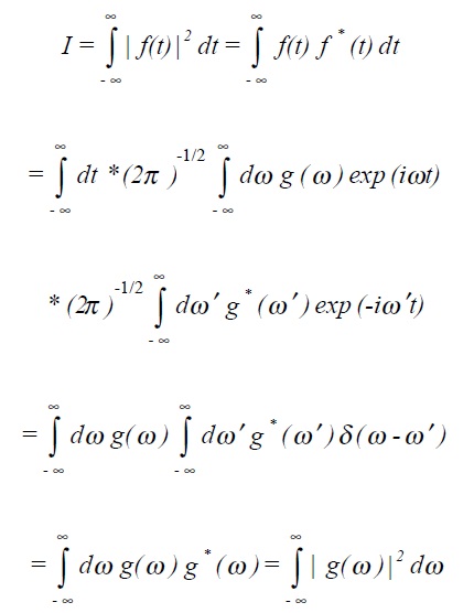
ιg(ω)ι2 is sometimes denoted as φtt (ω) or alternatively S(n) and is called the power density spectrum or power spectral density.
Example: Damped harmonic oscillator
ιg(ω)ι2 represents the energy (dissipated) per unit frequency. If σωn > > 1, then for ω ≈ωn
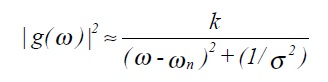
which can be recognised as the response of a damped harmonic oscillator to driving frequencies near to its resonant frequency.
Note that the term I, defined in section 5.4 is the mean square value (or variance) of the function (often a time series). In other words the area under a power spectral density function S(n) is simply the variance.
It is often found convenient to plot S(n) against the logarithm of frequency. In order to preserve the equivalence of areas under the curve with contributions to the variance, the y-axis is chosen as n S(n).
6.5. Frequency response, convolution and deconvolution
For a linear system with transfer function G(s) we can examine the response of the system
to a sinusoidal input u(t) = sin (ωt) using the techniques developed in section 3.
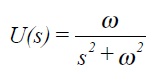
The output C(s) = G(s) U(s). Taking a ratio of suitable polynomial expansions for G(s) and using partial fractions to express C(s) gives
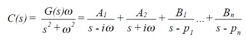
where, it can be recalled, the pi are the poles of the system (roots of the characteristic equation), and Ai, Bi are simply constants.
Taking inverse Laplace transforms gives
![]()
The first two terms represent the particular integral (often referred to as the steady state response) and the remaining terms represent the complementary function (the transient response).
Assuming all the poles pi have negative real ports (true for stable systems) the transient terms tend to zero as t tends to infinity, thus only the first two terms remain, ie
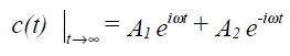
A1 and A2 can be determined by multiplying C(s) by (s - iω) and (s + iω) respectively and then setting s = iω and s = - iω.
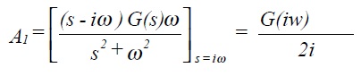
Similarly A2 = G(-iω)/-2i
Written in magnitude and phase terms (ratio of steady state output to input amplitude, and phase shift between output and input sin functions).
![]()
In other words the magnitude and phase components of a systems frequency response is obtained by replacing s with iω in the transfer function and taking the modulus and argument of the result.
If a system is exposed to a signal with a known spectral density X(ω), the output spectra density can be shown to be given by
![]()
where ιG (iω)ι2 is sometimes written as H(ω).
If f(x) and g(x) are two functions, the convolution, written f * g is defined to be
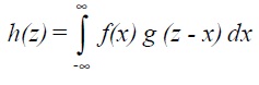
Note that if g is the delta-function, then h(z) = f(z).
The Fourier transform of the product of two functions is the convolution of the separate Fourier transforms multiplied by (2π )−1/ 2 .

7. Matrices and Eigen Value Analysis
Why?
Wind turbines are examined as dynamic systems in Wind II and these notes provide the basis of dynamic analysis. You will not however be expected to manipulate matrices as part of the course.
What?
Notation:
Matrices are denoted by bold capitals, A, M; while elements/components of matrix are denoted by lower case with subscripts.
For example:
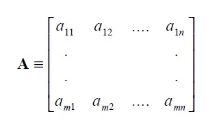
is an m by n matrix, (m x n).
Lower case bold is used for column or row vectors (matrices with one of the dimensions equal to unity), eg u, v, x y.
For square matrices:
The determinant of M (det M) is written ιMι
The transpose of A is AT, ie aij ↔aji
M is singular if ιMι= 0, otherwise non-singular
Inverse of A for non-singular matrices is denoted A-1 such that AA-1= , the unit matrix .
A matrix M is symmetric if MT = M
If MT = -M, then the matrix is skew-symmetric.