Maths
1. Why do I need maths?
2. Taylor series
3. Complex numbers
4. Differential equations and Laplace transform
5. State space analysis
6. Fourier transform and spectral density functions
7. Matrices and Eigen value analysis
8. Statistics and applied probability
4. Differential Equations and the Laplace Transform
4.3. The Laplace transform
The Laplace transform is an integral transform given by
![]()
It is a linear transformation which takes x to a new, in general, complex variable s. It is used to convert differential equations into purely algebraic equations.
Some examples are given in the table below:
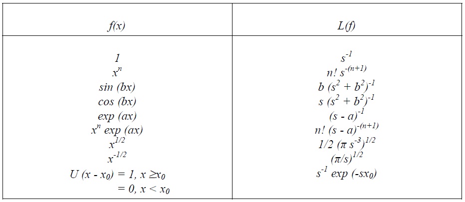
Deriving the inverse transform is problematic. It tends to be done through the use of tables
of transforms such as the one above.
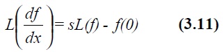
For application to differential equations we start by evaluating L(df/dx) using integration by
parts, the result is
This process can be repeated for ![]() etc, giving
etc, giving
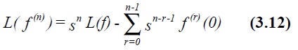
Hence the Laplace transform of any derivative can be expressed in terms of L(f) plus derivatives evaluated at x = 0. It is thus possible to rewrite any differential equation in terms of an algebraic equation for L(y).
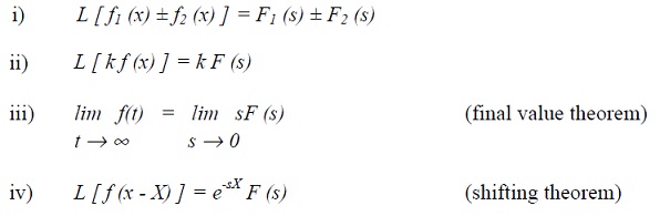
Four useful properties of Laplace transforms can be established.
4.3.1 Control theory applications
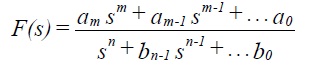
Laplace transforms are widely used in classical control theory. The independent variable is often taken as time t. In many applications the transformed differential equation will turn out to be the ratio of two polynomials in s, for example
If required this can be split by partial fractions to give
![]()
where the inverse transform L-1 can be found separately for each element. Hence
![]()
Often in control theory the inverse transform is not taken since much can be concluded (regarding stability etc) from the form of F(s).
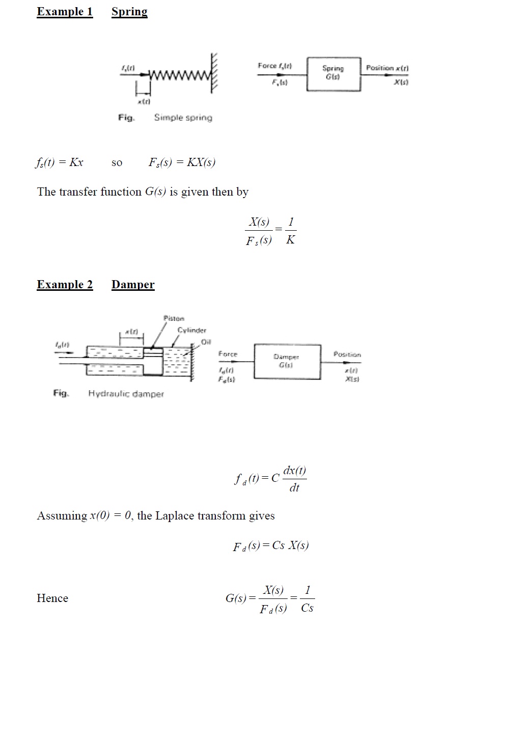
The transfer function of a linear system is defined as the ratio of the Laplace transform of the output of the system to the Laplace transform of the input to the system. It is denoted by G(s) or H(s). The linear assumption means that the properties of the system (eg G(s)) are not dependent on the state of the system (value of t or s).
For transfer functions, the initial conditions are assumed to be zero so that
![]()
Differential equations are transformed into the Laplace domain simply by replacing ![]() etc. The resulting transfer function can then be written
etc. The resulting transfer function can then be written
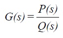
where P and Q are polynomials in s. The properties of G are determined by the roots of Q (s) = 0 (which is known as the characteristic equation).
NB. These roots are referred to as poles of the system since G(s) becomes infinite at these values of s. The order of the system is the order of Q(s).
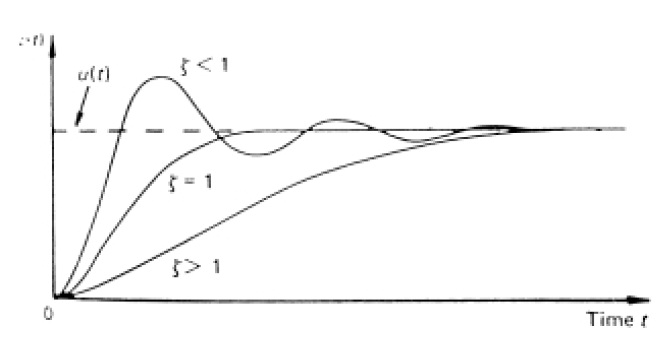
4.3.2 Calculating transient response to a step input
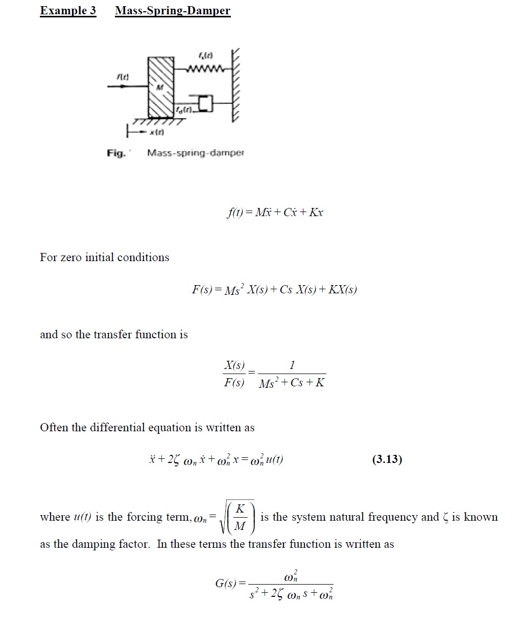
The approach developed above can be used to calculate the transient response of linear systems. First order systems are straightforward to analyse but not particularly interesting. We will concentrate here on second order systems.
The output of a system is often denoted by c(t) and its Laplace transform by C(s) with the
input being u(t) and U(s) respectively.
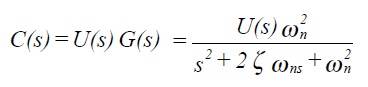
The Laplace transform of a step input is 1/s and so
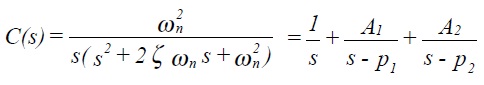
using partial fractions where A1 and A2 are constants and p1 and p2 are the roots of the characteristic equation. Hence, taking inverse transforms,

The nature of the response depends on the nature of the roots, which is determined by the damping factor ζ. The figure below shows the form of step response for a second order system.