
Maths
1. Why do I need maths?
2. Taylor series
3. Complex numbers
4. Differential equations and Laplace transform
5. State space analysis
6. Fourier transform and spectral density functions
7. Matrices and Eigen value analysis
8. Statistics and applied probability
6. Fourier Transform and Spectral Density Functions
6.1. Fourier transforms
The Fourier transform (or Fourier integral) is obtained formally be allowing the period T of the Fourier series to become infinite. Instead of only integer frequency contributions (as in the Fourier series) a continuous function of frequency results. From equation (5.1) we can write down
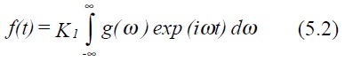
where K1 is an arbitrary constant. By analogy, the Fourier coefficients Cn become a continuous function g(ω), ie
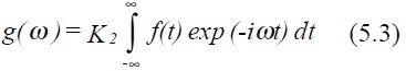
K2 is also arbitrary, although the product K1 K2 is fixed. It is conventional to take K1 and K2 as 1/ 2π .
Equation (5.3) is known as the Fourier transform and (5.2) the inverse Fourier transform.
The function g(ω) is called the spectrum of f(t).
It can be noted that as an integral transform it is similar to the Laplace transform but that both limits of integration are infinite.
Example 1: Fourier transform of exponential decay function f(t) = 0 for t < 0 and f(t) = exp (-λt) for t≥ 0 with λ > 0.
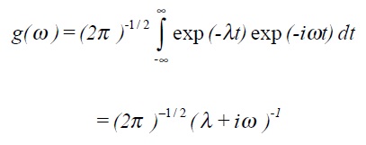
NB: Complex contour integration is required to derive this, however it is easily checked using the inverse transform.
Example 2: Fourier transform of Gaussian or normal distribution function, (zero mean and standard deviation σ).
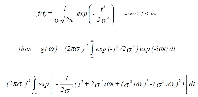
which can be rewritten as
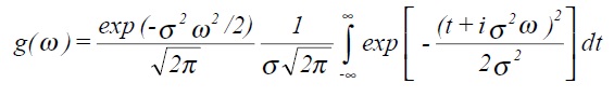
Finally this can be shown to give
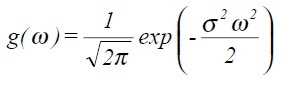
which is also a Gaussian distribution with zero mean but with standard deviation equal to 1/σ.
ie σω σt = 1
The narrower in time an impulse is, the greater the spread of frequency components.