
Maths
1. Why do I need maths?
2. Taylor series
3. Complex numbers
4. Differential equations and Laplace transform
5. State space analysis
6. Fourier transform and spectral density functions
7. Matrices and Eigen value analysis
8. Statistics and applied probability
6. Fourier Transform and Spectral Density Functions
6.4. Parseval's theorem
Parseval's theorem can be stated as:
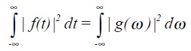
Its proof regimes use the properties of the δ-function.
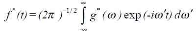
In brief, if we take the complex conjugate of (5.2), the inverse transform
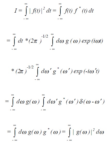
The intensity I of a function is defined to be
ιg(ω)ι2 is sometimes denoted as φtt (ω) or alternatively S(n) and is called the power density spectrum or power spectral density.
Example: Damped harmonic oscillator
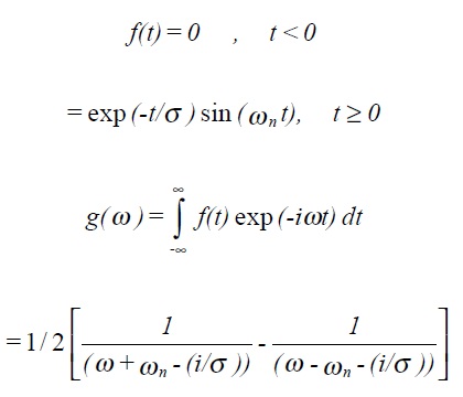
ιg(ω)ι2 represents the energy (dissipated) per unit frequency. If σωn > > 1, then for ω ≈ωn
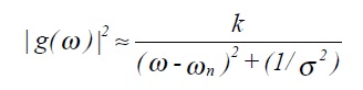
which can be recognised as the response of a damped harmonic oscillator to driving frequencies near to its resonant frequency.
Note that the term I, defined in section 5.4 is the mean square value (or variance) of the function (often a time series). In other words the area under a power spectral density function S(n) is simply the variance.
It is often found convenient to plot S(n) against the logarithm of frequency. In order to preserve the equivalence of areas under the curve with contributions to the variance, the y-axis is chosen as n S(n).