For a linear system with transfer function G(s) we can examine the response of the system
to a sinusoidal input u(t) = sin (ωt) using the techniques developed in section 3.

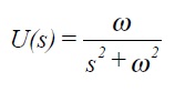
The output C(s) = G(s) U(s). Taking a ratio of suitable polynomial expansions for G(s) and using partial fractions to express C(s) gives

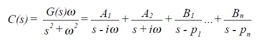
where, it can be recalled, the pi are the poles of the system (roots of the characteristic equation), and Ai, Bi are simply constants.

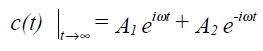
Taking inverse Laplace transforms gives

The first two terms represent the particular integral (often referred to as the steady state response) and the remaining terms represent the complementary function (the transient response).

Assuming all the poles pi have negative real ports (true for stable systems) the transient terms tend to zero as t tends to infinity, thus only the first two terms remain, ie

A1 and A2 can be determined by multiplying C(s) by (s - iω) and (s + iω) respectively and then setting s = iω and s = - iω.

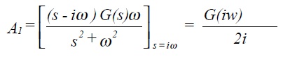
Similarly A₂ = G(-iω)/-2i

Written in magnitude and phase terms (ratio of steady state output to input amplitude, and phase shift between output and input sin functions).

In other words the magnitude and phase components of a systems frequency response is obtained by replacing s with iω in the transfer function and taking the modulus and argument of the result.

If a system is exposed to a signal with a known spectral density X(ω), the output spectra density can be shown to be given by

where ιG (iω)ι² is sometimes written as H(ω).

If f(x) and g(x) are two functions, the convolution, written f * g is defined to be

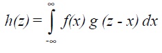
Note that if g is the delta-function, then h(z) = f(z).

The Fourier transform of the product of two functions is the convolution of the separate Fourier transforms multiplied by (2π )^{−1/ 2} .